Welcome
Today we will have a look at instrumental variables. We will explore encouragement experimental designs and how IVs can be used in observational data settings. Additionally, we will learn how to calculate our LATE manually with the wald estimator and in R with two-stage square least regressions through ivreg
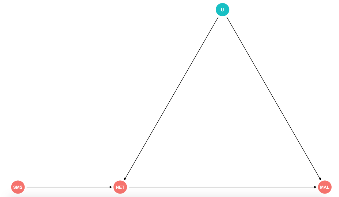
Measuring the effect of mosquito net use on malaria infection
Imagine that the organization you work for is laying out a project to distribute mosquito nets to help combat malaria transmitions. You are in charge of running the impact evaluation of this program. You realize that it is unethical to randomize who receives the nets, so you consider an encouragement design. You decide to randomly select five villages out of the ten to send SMS reminders every night encouraging them to use the mosquito nets. (This example is using simulated data)
Assumptions
For this evaluation to render credible results we need to fulfill a certain set of assumtions:
a) Relevance: Also known as non-zero average encouragement effect. Does our \(Z\) create variation in our \(D\)? In other words, is the mosquito net use different under the encouragement group? (Statistically testable)
b) Exogeneity/Ignorability of the instrument: Potential outcomes and treatments are independent of \(Z\). In this case given by out randomization of encouragement by villages.
c) Exclusion restriction: The instrument only affects the outcome via the treatment. In other words, there are no alternative paths through which our SMS can have an effect on malaria infections other that the use of the mosquito nets.
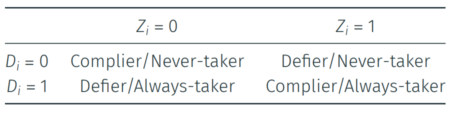
d) Monotonicity: No defiers. We assume that non-compliers fall in the camp of always- and never-takers. We would not expect subjects who when encouraged would not use the nets, but would use them if they did not recieve the SMS reminder.
loading our packages and data
library(dplyr) # for data wrangling
library(readr) # for loading the .csv data
library(ggplot2) # for creating plots
library(summarytools) # for ctable()
library(stargazer) # for formatting model output
library(kableExtra) # for formatting data frames
library(AER) # for ivreg()
library(tidyr) # for pivot_wider()

set.seed(123) # for consistent results

eval_data <- readr::read_csv("https://raw.githubusercontent.com/seramirezruiz/stats-ii-lab/master/Session%205/data/evaluation_data.csv") # loading simulated data frame of the intervention
Exploring our results
You receive the results of your intervention from the M&E officers. This is what they look like:
summarytools::st_options(footnote = NA) # to get rid of the footnote of ctable
print(summarytools::ctable(eval_data$net_use, eval_data$sms, prop = "n"),
      method = "render") # include results = "asis" to view html in the knitted file
Cross-Tabulation
net_use * sms
Data Frame: eval_data| sms | |||
|---|---|---|---|
| net_use | 0 | 1 | Total |
| 0 | 335 | 110 | 445 |
| 1 | 165 | 390 | 555 |
| Total | 500 | 500 | 1000 |
a) Where are our compliers and non-compliers?
b) How many people were encouraged via SMS, but did not use the net?
c) How many people were not encouraged via SMS, yet they utilized the net?
We can also utilize dplyr to check the average malaria on each stratum:
eval_data %>%
  dplyr::group_by(net_use, sms) %>% #group our data on the tratment and instrument
  dplyr::summarize(avg = mean(malaria)) %>% #get the aveage value of malaria
  dplyr::mutate(avg = round(avg, 2)) %>% #round the avg to 2 decimal places
  tidyr::pivot_wider(names_from = sms, values_from = avg) %>% #convert to wide format
  knitr::kable() %>% #turn to kable
  kableExtra::kable_styling() %>%
kableExtra::add_header_above(c("", "sms" = 2)) #add header for sms| net_use | 0 | 1 |
|---|---|---|
| 0 | 0.73 | 0.55 |
| 1 | 0.05 | 0.08 |
Additionally, we can explore our data visually to check beyond compliance and see in which groups malaria was present. In this case, we are dealing with binary outcomes. That is, you can either be or not be infected, which are represented by the color dimension in different groups.
ggplot(eval_data, aes(x = factor(sms),
                      y = factor(net_use),
                      color = factor(malaria))) +
  geom_point() +
  geom_jitter() +
  theme_minimal() +
  scale_x_discrete(labels = c("SMS = 0", "SMS = 1")) +
  scale_y_discrete(labels = c("NET = 0", "NET = 1")) +
  scale_color_discrete(labels = c("Not infected", "Infected")) +
  labs(x = "Encouragement",
       y = "Treatment",
       color = "")
Exploring our set-up
Let's check whether SMS encouragement is a strong instrument
In other words, we are looking at the relevance assumption. Does our SMS encouragement create changes in our mosquito net use?
summary(lm(net_use ~ sms, eval_data))##
## Call:
## lm(formula = net_use ~ sms, data = eval_data)
##
## Residuals:
## Min 1Q Median 3Q Max
## -0.78 -0.33 0.22 0.22 0.67
##
## Coefficients:
## Estimate Std. Error t value Pr(>|t|)
## (Intercept) 0.33000 0.01984 16.64 <2e-16 ***
## sms 0.45000 0.02805 16.04 <2e-16 ***
## ---
## Signif. codes: 0 '***' 0.001 '**' 0.01 '*' 0.05 '.' 0.1 ' ' 1
##
## Residual standard error: 0.4436 on 998 degrees of freedom
## Multiple R-squared: 0.205, Adjusted R-squared: 0.2042
## F-statistic: 257.3 on 1 and 998 DF, p-value: < 2.2e-16Economists have established as a "rule-of-thumb" for the case of a single endogenous regressor to be considered a strong instrument should have a F-statistic 1 greater than 10. From this regression, we can see that SMS encouragement is a strong instrument. Additionally, the substantive read in this case is that only 33% of those who did not receive the SMS utilized the mosquito nets, where as 78% of those who got the SMS encouragement did.
Let's gather a naïve estimate of mosquito net use and malaria infection.
Also, why do you think we call this a naïve estimate?
naive_model <- lm(malaria ~ net_use, eval_data)
summary(naive_model)
##
## Call:
## lm(formula = malaria ~ net_use, data = eval_data)
##
## Residuals:
## Min 1Q Median 3Q Max
## -0.68315 -0.06847 -0.06847 0.31685 0.93153
##
## Coefficients:
## Estimate Std. Error t value Pr(>|t|)
## (Intercept) 0.68315 0.01722 39.67 <2e-16 ***
## net_use -0.61468 0.02312 -26.59 <2e-16 ***
## ---
## Signif. codes: 0 '***' 0.001 '**' 0.01 '*' 0.05 '.' 0.1 ' ' 1
##
## Residual standard error: 0.3633 on 998 degrees of freedom
## Multiple R-squared: 0.4147, Adjusted R-squared: 0.4141
## F-statistic: 707 on 1 and 998 DF, p-value: < 2.2e-16
Let's gather our intent-to-treat effect (ITT)
This is the effect that our SMS encouragement had on malaria infections. \(ITT = E(Malaria_i|SMS=1) - E(Malaria_i|SMS=0)\). What does this tell us?
itt_model <- lm(malaria ~ sms, eval_data)
summary(itt_model)
##
## Call:
## lm(formula = malaria ~ sms, data = eval_data)
##
## Residuals:
## Min 1Q Median 3Q Max
## -0.504 -0.180 -0.180 0.496 0.820
##
## Coefficients:
## Estimate Std. Error t value Pr(>|t|)
## (Intercept) 0.50400 0.01996 25.25 <2e-16 ***
## sms -0.32400 0.02823 -11.48 <2e-16 ***
## ---
## Signif. codes: 0 '***' 0.001 '**' 0.01 '*' 0.05 '.' 0.1 ' ' 1
##
## Residual standard error: 0.4463 on 998 degrees of freedom
## Multiple R-squared: 0.1166, Adjusted R-squared: 0.1157
## F-statistic: 131.8 on 1 and 998 DF, p-value: < 2.2e-16
Let's gather out local average treatment effect (LATE)
We have several options for this:
- Wald Estimator We can calculate this by hand. Let's try that now, using the values from the table. We can also calculate the average malaria rates among those who did and did not receive an SMS (no SMS = 0.504, yes SMS = 0.18). \[LATE = \frac{cov(Y_i,Z_i)}{cov(D_i,Z_i)}\]
| sms | |||
|---|---|---|---|
| net_use | 0 | 1 | Total |
| 0 | 335 | 110 | 445 |
| 1 | 165 | 390 | 555 |
| Total | 500 | 500 | 1000 |
Let's take a look at our numerator \(cov(Y_i,Z_i)\)
\(E(Y|Z = 1)\) = 0.18
\(E(Y|Z = 0)\) = 0.504
Let's take a look at our denominator \(cov(D_i,Z_i)\)
\(E(D ∣ Z = 1) = \frac{390}{(390 + 110)} = 0.78\)
\(E(D ∣ Z = 0) = \frac{165}{(165 + 335)} = 0.33\)
We can calculate our LATE \[LATE = \frac{(0.18 - 0.504)}{(0.78 - 0.33)} = -0.72\]
- Two-stage Least Squares (2SLS). We will learn how to do this with ivreg(), which is part of the
AERpackage. It fits instrumental-variable regression through two-stage least squares. The syntax is the following:
late_model <- AER::ivreg(malaria ~ net_use | sms, data = eval_data)
summary(late_model)
##
## Call:
## AER::ivreg(formula = malaria ~ net_use | sms, data = eval_data)
##
## Residuals:
## Min 1Q Median 3Q Max
## -0.7416 -0.0216 -0.0216 0.2584 0.9784
##
## Coefficients:
## Estimate Std. Error t value Pr(>|t|)
## (Intercept) 0.74160 0.03089 24.00 <2e-16 ***
## net_use -0.72000 0.05159 -13.96 <2e-16 ***
## ---
## Signif. codes: 0 '***' 0.001 '**' 0.01 '*' 0.05 '.' 0.1 ' ' 1
##
## Residual standard error: 0.3671 on 998 degrees of freedom
## Multiple R-Squared: 0.4025, Adjusted R-squared: 0.4019
## Wald test: 194.8 on 1 and 998 DF, p-value: < 2.2e-16
Mechanics behing two-stage least squares (2SLS)
What ivreg() is doing in the background is the following:
net_use_hat <- lm(net_use ~ sms, eval_data)$fitted.values # get fitted values from first stage (the part of x that is exogenously driven by z)
summary(lm(eval_data$malaria ~ net_use_hat)) # run second stage with instrumented x (careful, the standard errors are wrong; better use ivreg() from AER instead)
##
## Call:
## lm(formula = eval_data$malaria ~ net_use_hat)
##
## Residuals:
## Min 1Q Median 3Q Max
## -0.504 -0.180 -0.180 0.496 0.820
##
## Coefficients:
## Estimate Std. Error t value Pr(>|t|)
## (Intercept) 0.74160 0.03757 19.74 <2e-16 ***
## net_use_hat -0.72000 0.06273 -11.48 <2e-16 ***
## ---
## Signif. codes: 0 '***' 0.001 '**' 0.01 '*' 0.05 '.' 0.1 ' ' 1
##
## Residual standard error: 0.4463 on 998 degrees of freedom
## Multiple R-squared: 0.1166, Adjusted R-squared: 0.1157
## F-statistic: 131.8 on 1 and 998 DF, p-value: < 2.2e-16
Thinking about the validity of instruments
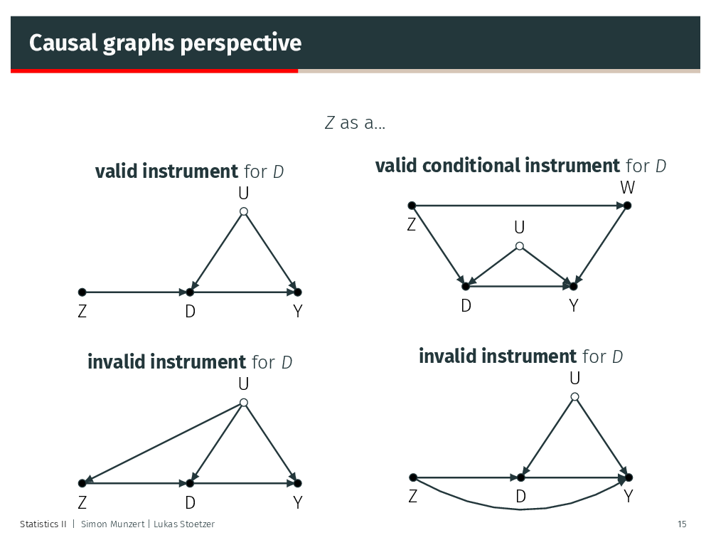
We can also adapt the ivreg() syntax to accomodate valid conditional instruments:
An F statistic is a value you get when you run an ANOVA test or a regression analysis to find out if the means between two populations are significantly different. It’s similar to a t-statistic from a t-test; A-T test will tell you if a single variable is statistically significant and an F test will tell you if a group of variables are jointly significant.↩