Data
The Comparative Legislators Database (CLD) is a one-stop shop for rich, diverse and integrated individual-level data on national political representatives. The database contains information for over 45,000 contemporary and historical legislators from 14 countries and the European Parliament. In our project, we unite collaborative micro-data collection efforts. We bring these together through the use of Wikipedia and Wikidata.
Data access
There are multiple ways to access the data depending your use-case. You can download individual .csv files for individual legislatures, generate SQL queries to gather specific information from the database, and finally use the legislatoR package for the software environment R.
Below you will find an overview of our current coverage and other databases that the CLD can be integrated with:
| Country | Legislative sessions | Politicians (unique) | Integrated with | CSV |
|---|---|---|---|---|
| Austria (Nationalrat) | all 27 (1920-2019) |
1,923 | ParlSpeech V2 (Rauh/Schwalbach 2020) | |
| Canada (House of Commons) | all 43 (1867-2019) |
4,515 | ||
| Czech Republic (Poslanecka Snemovna) | all 8 (1992-2017) |
1,020 | ParlSpeech V1 (Rauh et al. 2017) | |
| France (Assemblée) | all 15 (1958-2017) |
3,933 | ||
| Germany (Bundestag) | all 19 (1949-2017) |
4,075 | BTVote data (Bergmann et al. 2018), ParlSpeech V1 (Rauh et al. 2017), Reelection Prospects data (Stoffel/Sieberer 2017) |
|
| Ireland (Dail) | all 33 (1918-2020) |
1,408 | Database of Parliamentary Speeches in Ireland (Herzog/Mikhaylov 2017) | |
| Scotland (Parliament) | all 5 (1999-2016) |
305 | ParlScot (Braby/Fraser 2021) | |
| Spain (Congreso de los Diputados) | all 14 (1979-2019) |
2634 | ParlSpeech V2 (Rauh/Schwalbach 2020) | |
| United Kingdom (House of Commons) | all 58 (1801-2019) |
13,215 | EggersSpirling data (starting from 38th session, Eggers/Spirling 2014), ParlSpeech V1 (Rauh et al. 2017) |
|
| United States (House and Senate) | all 116 (1789-2019) |
12,512 | Voteview data (Lewis et al. 2019), Congressional Bills Project data (Adler/Wilkserson 2018) |
|
| 10 | 338 | 45,540 | 12 |
Structure
The CLD comes as a relational database. This means that all tables can be joined with the Core table via one of two keys - the Wikipedia page ID or the Wikidata ID. These keys uniquely identify individual politicians. The figure below illustrates this structure and the CLD's content.
For each legislature, the CLD holds nine tables:
- Core (sociodemographic data)
- Political (political data)
- History (full revision records of individual Wikipedia biographies)
- Traffic (daily user traffic on individual Wikipedia biographies starting from July 2007)
- Social (social media handles and personal website URLs)
- Portraits (URLs to portraits)
- Offices (public offices)
- Professions (professions)
- IDs (identifiers linking politicians to other files, databases, or websites)
The tables contain the following variables (see respective R help files for further details):
- Core: Country, Wikipedia page ID, Wikidata ID, Wikipedia Title, full name, sex, ethnicity, religion, date of birth and death, place of birth and death.
- Political: Wikipedia page ID, legislative session, party affiliation, lower constituency, upper constituency, constituency ID, start and end date of legislative session, period of service, majority status, leader positions.
- History: Wikipedia page ID, Wikipedia revision and previous revision ID, editor name/IP and ID, revision date and time, revision size, revision comment.
- Traffic: Wikipedia page ID, date, user traffic.
- Social: Wikidata ID, Twitter handle, Facebook handle, Youtube ID, Google Plus ID, Instagram handle, LinkedIn ID, personal website URL.
- Portraits: Wikipedia page ID, Wikipedia portrait URL.
- Offices: Wikidata ID, a range of offices such as attorney general, chief justice, mayor, party chair, secretary of state, etc.
- Professions: Wikidata ID, a range of professions such as accountant, farmer, historian, judge, mechanic, police officer, salesperson, teacher, etc.
- IDs: Wikidata ID, IDs for integration with various political science datsets as well as a range of other IDs such as parliamentary website IDs, Library of Congress or German National Library IDs, Notable Names Database or Project Vote Smart IDs, etc.
Note that for some legislatures or legislative periods, tables may only hold information for a subset of politicians or variables. In successive versions of the CLD, we fill some of these gaps.
legislatoR
legislatoR is a package for the software environment R that facilitates access to the Comparative Legislators Database (CLD). The package is available through CRAN and GitHub. To install the package from CRAN, type:
install.packages("legislatoR")You can also download the development version directly from Github:
# install.packages("devtools")
devtools::install_github("saschagobel/legislatoR")
Usage
A working Internet connection is required to access the CLD in R. This is because the data are stored online and not installed together with the package. The package provides table-specific function calls. These functions are named after the respective table and preceded by legislatoR::get_. To fetch the Core table, use the legislatoR::get_core() function, for the Political table, use the legislatoR::get_political() function. Call the package help file via ?legislatoR() to get an overview of all function calls. Tables are legislature-specific, so a letter country code must be passed as an argument to the function. Here is a breakdown of all country codes. You can also call the legislatoR::cld_content() function to get an overview of the CLD's scope and valid country codes.
| Legislature | Code | Legislature | Code | Legislature | Code |
|---|---|---|---|---|---|
| Austrian Nationalrat | aut |
German Bundestag | deu |
UK House of Commons | gbr |
| Canadian House of Commons | can |
Irish Dail | irl |
United States Congress | usa_house/usa_senate |
| Czech Poslanecka Snemovna | cze |
Scottish Parliament | sco |
||
| French Assemblée | fra |
Spanish Congreso | esp |
Working with the legislatoR package in R
The legislatoR package provides an easy-to-use interface to the CLD in R. This brief tutorial will present two use-cases to illustrate how to engage the different tables of the database to extract information for analyses. To be precise, we will:
- explore the distribution of seats in the U.S. Senate during the 116th United States Congress (Jan 2019 - Jan 2021)
- map the birthplaces of all the members of the Bundestag by political party
# load the libraries
library(legislatoR)
library(dplyr) #data manipulation
library(ggplot2) #data visualization
library(ggtext) #text aesthetics in ggplot2
library(ggpol) #geom_parliament() (parliament plots)
library(sf) #spatial vector encodings in R
library(rnaturalearth) #natural earth map data
library(rnaturalearthdata) #natural earth map data

set.seed(1310) # to get consistent results from randomization
The U.S. Senate during the 116th United States Congress
The Core table is at the center of the database structure. This table contains basic demographic information about the legislators, in addition to the joining keys: Wikipedia page ID (pageid) and the Wikidata ID (wikidataid). These data can be retrieved through the get_core() call function. The call functions take the legislature code as an argument (i.e., get_*(legislature="code")). Each table can be called independently based on the use-case and can be linked through one of the joining keys.
legislatoR::get_core(legislature = "usa_senate") %>% # load US Senate core
    dplyr::sample_n(10) #get ten random entries
In this case, we will employ Political table to derive the counts of the seats each party held:
# load US Senate political table for the 116th Congress
us_senate_political <- legislatoR::get_political(legislature = "usa_senate") %>%
  dplyr::filter(session == 116) #filter only legislators from the 116th Congress

dplyr::sample_n(us_senate_political, 10) #print ten random entries
You can employ dplyr verbs to extract the seat counts per party and generate a visual illustration of the distribution:
# get the seat counts per party for parliament plot
us_senate_counts <- us_senate_political %>%
  dplyr::group_by(party) %>% #nest at party
  dplyr::summarize(seats = n()) %>% #generate counts
  dplyr::mutate(colors = dplyr::case_when(party == "D" ~ "#3885D3",
                                          party == "R" ~ "#E02E44",
                                          party == "Independent" ~ "#637684")) #assign party colors for visualization

us_senate_counts
We can use the us_senate_counts data frame as the input for our plot:
# a caption with some md formating
caption_plot <- paste0("The 116th US Senate was controlled by the <b style='color:#E02E44'> Republican party</b> with <b style='color:#E02E44'>",
                       us_senate_counts$seats[us_senate_counts$party == "R"], # Number of Republican seats
                       " seats</b>.<br>The <b style='color:#3885D3'>Democratric party</b> held <b style='color:#3885D3'>",
                       us_senate_counts$seats[us_senate_counts$party == "D"], # Number of Democrat seats
                       " seats</b>. The <b style='color:#637684'>",
                       us_senate_counts$seats[us_senate_counts$party == "Independent"], # Number of Independent seats
                       " Independents </b>caucased with the Democrats."
)

# plot parliament seats
ggplot(us_senate_counts) +
  ggpol::geom_parliament(aes(seats = seats, fill = party), color = "black") +
  scale_fill_manual(values = us_senate_counts$colors, labels = us_senate_counts$party) +
  coord_fixed() +
  labs(title = "<b>US Senate membership (116th Congress)</b>",
       caption = caption_plot) +
  theme_void() +
  theme(legend.position = "none",
        plot.title = ggtext::element_markdown(),
plot.caption = ggtext::element_markdown()) 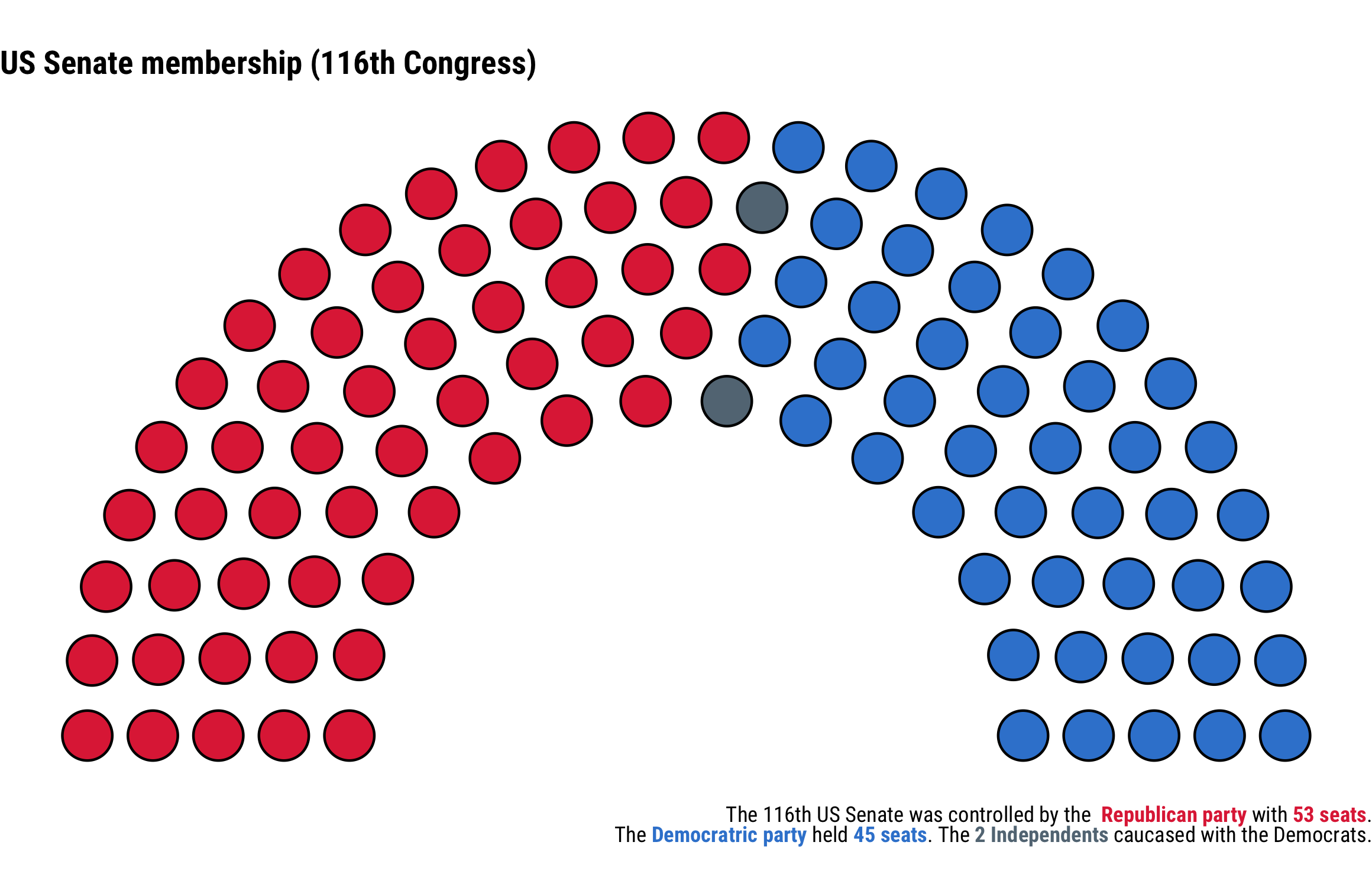
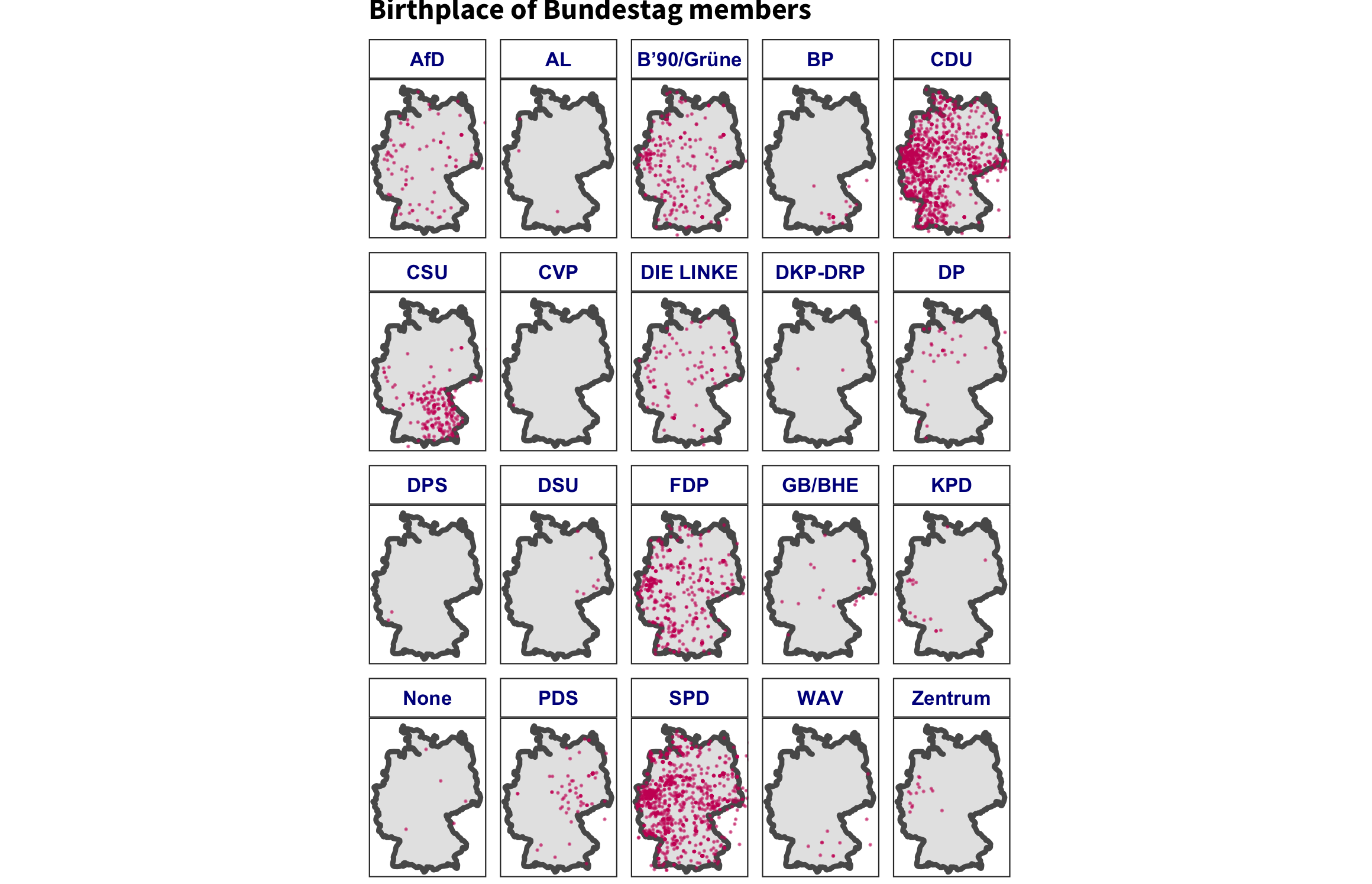
The birthplaces of German parlimentarians
In most instances, you will need to link information from different tables in the database. For instance, in this case we need the parliamentarians' birthplace coordinates and their political party. These two data points are in the Core and Political tables. One easy way to link the tables is by employing dplyr joins.
# assign Political and Core tables to the environment
deu_politicians <- dplyr::left_join(x = legislatoR::get_political(legislature = "deu"),
                                    y = legislatoR::get_core(legislature = "deu"),
                                    by = "pageid") #these two tables can be joined through their Wikipedia page ID

head(deu_politicians) #print first couple observationsThe deu_politicians data frame contains all the information from the two tables. We can use these data to extract the latitudes and longitudes of the legislators' birthplace for a map.
# extract birthplace latitudes and longitudes with regular expressions
deu_birthplace_map_df <- deu_politicians %>%
  dplyr::distinct(wikidataid, .keep_all = T) %>% # keep unique entries of legislators
  dplyr::mutate(lat = stringr::str_extract(birthplace, "[-[:digit:]]{1,4}\\.[:digit:]+") %>% as.numeric(),
                lon = stringr::str_extract(birthplace, "[-[:digit:]]{1,4}\\.[:digit:]+$") %>% as.numeric())

# define German boundaries
lat1 <- 47; lat2 <- 55.5 ; lon1 <- 5.5; lon2 <- 15.5

germany_sf <- rnaturalearth::ne_countries(scale = "medium", returnclass = "sf", country = "Germany") #get spatial encodings for Germany

ggplot(germany_sf) +
  geom_sf(size = 1) +
  geom_point(data = deu_birthplace_map_df, aes(x = lon, y = lat), size = .25,
             shape = 20, color = "#cc0065", alpha = 0.5) +
  theme_bw() +
  facet_wrap(~party) +
  coord_sf(xlim = c(lon1, lon2), ylim = c(lat1, lat2), expand = FALSE) +
  labs(title = "<b>Birthplace of Bundestag members<b>")+
  theme(plot.margin=grid::unit(c(0,0,0,0), "mm"),
        axis.title = element_blank(),
        axis.ticks = element_blank(),
        axis.text=element_blank(),
        panel.grid.major = element_blank(),
        panel.grid.minor = element_blank(),
        legend.position = "none", text = element_text(size=10),
        panel.grid.minor.y =  element_blank(),
        strip.background = element_rect(fill="white"),
        strip.text.x = element_text(color = "darkblue", face = "bold"),
        plot.title = ggtext::element_markdown(family = "Source Sans Pro"))